Row Selection Using Slicers in PowerPivot - Part 2
Reposted from Jason Thomas blog with the author's permission.
This post is a continuation of the Row Selection Using Slicers in PowerPivot – Part 1 (so it might be a good idea to read that post before this). In our last post, we discussed the basic solution pattern for row selection using slicers in PowerPivot. In this post, we will discuss two other scenarios which are slightly more complex but still uses the same pattern.
Scenario III - GroupNames in multiple dimensions
Our data model for this scenario will have a Product table, a Customer table and a Fact table which shows the sales by Product and Customer. The requirement is to select either Product or Customer in the slicer and display the appropriate rows in the pivot table.
1) As per the solution steps, we first have to create the Group table
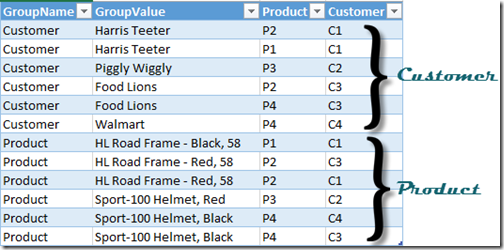
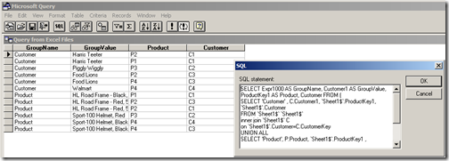
Note that we need two grain columns here, as the GroupNames belong to two dimensions – Product and Customer. The GroupName will be Customer and Product, and the GroupValues will be the actual product or customer values depending on the GroupName. As with the previous posts, I use MS Query to generate this table.
SELECT Expr1000 AS GroupName, Customer1 AS GroupValue, ProductKey1 AS Product, Customer FROM
(
SELECT 'Customer' , C.Customer1, `Sheet1$`.ProductKey1, `Sheet1$`.Customer
FROM `Sheet1$` `Sheet1$`
INNER JOIN `Sheet1$` C
ON `Sheet1$`.Customer=C.CustomerKey
UNION ALL
SELECT 'Product', P.Product, `Sheet1$`.ProductKey1 , `Sheet1$`.Customer
FROM `Sheet1$` `Sheet1$`
INNER JOIN `Sheet1$` P
ON `Sheet1$`.ProductKey1=P.ProductKey
)
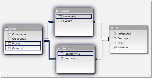
2) Add this new table (Group) to the data model and then relate the Product & Customer column in this table to the ProductKey column in the Product table & CustomerKey column in the Customer table.
3) Hide the original measure Sales, and then create a new measure with the formula given below
NewSales:=CALCULATE(SUM(Fact[Sales]), 'Group')
4) Check out the results by creating a pivot table with GroupValue on the rows, NewSales on Values and GroupName in Slicers.
Download the Excel 2013 file with the solution from here.
Scenario IV – Hybrid Scenario
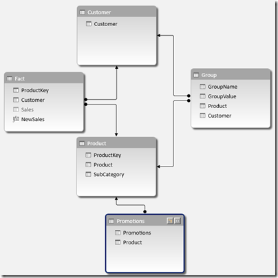
In this scenario, we are going to combine all the different scenarios we discussed till now and see how to handle that. The data model for this scenario will contain a Fact table which shows sales by Product and Customer, a Product table with the Product and SubCategory information, a Customer table and a Promotions table which has a many to many relationship with Product. The requirement is to have SubCategory (Scanario I), Promotions (Scenario II) and Customer (Scenario III) on slicers.
1) As usual, the first step is to generate the Group table.
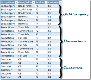
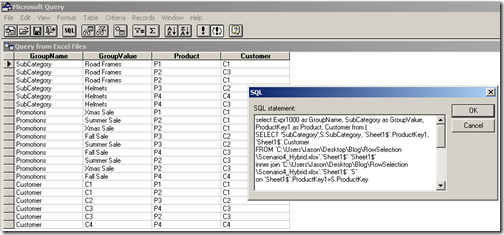
Note that even though we have only 4 subcategories, we end up with 6 rows because we will have to ensure that the grain is at a Product and Customer level. Similarly, we end up with 9 rows for Promotions when we convert the granularity of the Promotions table from just Product to the Product and Customer level. Find below the MS Query way of generating this table
SELECT Expr1000 AS GroupName, SubCategory AS GroupValue, ProductKey1 AS Product, Customer FROM
(
SELECT 'SubCategory',S.SubCategory, `Sheet1$`.ProductKey1, `Sheet1$`.Customer
FROM `C:UsersJasonDesktopBlogRowSelectionScenario4_Hybrid.xlsx`.`Sheet1$` `Sheet1$`
INNER JOIN `C:UsersJasonDesktopBlogRowSelectionScenario4_Hybrid.xlsx`.`Sheet1$` `S`
ON `Sheet1$`.ProductKey1=S.ProductKey
UNION ALL
SELECT 'Promotions',P.Promotions, P.Product1, S.Customer
FROM `C:UsersJasonDesktopBlogRowSelectionScenario4_Hybrid.xlsx`.`Sheet1$` `P`
INNER JOIN `C:UsersJasonDesktopBlogRowSelectionScenario4_Hybrid.xlsx`.`Sheet1$` `S`
ON P.Product1=S.ProductKey1
UNION ALL
SELECT 'Customer', Customer, ProductKey1, Customer
FROM `C:UsersJasonDesktopBlogRowSelectionScenario4_Hybrid.xlsx`.`Sheet1$`
WHERE Customer IS NOT NULL
)
2) Add this new table (Group) to the data model and then relate the Product & Customer column in this table to the ProductKey column in the Product table & CustomerKey column in the Customer table.
3) Hide the original measure Sales, and then create a new measure with the formula given below
NewSales:=CALCULATE(sum(Fact[Sales]), 'Group', Promotions)
Also note the use of the Promotions table (which is the many to many table) in the filter part of the calculate statement.
4) Check out the results by creating a pivot table with GroupValue on the rows, NewSales on Values and GroupName in Slicers.
Download the Excel 2013 file with the solution from here.
With that, we come to the end of this 2 part series on how to change the rows using slicers in PowerPivot. As you would have seen, the bulk of the work lies in generating the Group table and the rest is pretty simple. Hope these scenarios will help you in case you ever need to do the same.
 | Jason has been working with Microsoft BI tools since he joined the IT industry in 2006. Since then he has worked across SSAS, SSRS and SSIS for a large number of clients like Unilever, Imperial Tobacco, IATA, Schneider Electric, etc. He is currently working at MindTree Ltd, Bangalore (www.mindtree.com) and his personal blog site can be found at http://www.sqljason.com His blogs can also be found at the popular technical site BeyondRelational.com at http://beyondrelational.com/blogs/jason |

