Using The CubeSet() Function to Combine Selections From Multiple Slicers in Excel Power Pivot Reports

Reposted from Chris Webb's blog with the author's permission.

Since my last post on the Excel cube functions proved to be very popular, I thought I’d write a follow-up that shows off some more little-known but interesting functionality: how to use the CubeSet() function to combine selections from multiple slicers.

The Problem

Consider the following Power Pivot model based on data from the Adventure Works DW database:

The Internet Sales table contains one row per sales transaction; Product and Date are dimension tables that provide more information on the product bought in the transaction and the date the order was taken on. There’s one measure called Distinct Customers that returns the distinct count of customers; its definition is as follows:

Distinct Customers:=DISTINCTCOUNT('Internet Sales'[CustomerKey])

With this model you could build the following simple report by converting a PivotTable to cube functions:

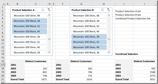
Obviously this will tell you how many distinct customers bought the products selected in the slicer each year. You could also duplicate the slicer and the cube functions and have two reports side-by-side so you could compare the number of customers that bought two different groups of products:

The question here is, though, how can you create a third report that shows the number of distinct customers that bought any of the products selected across both slicers? So, using the example above, the report on the left shows the number of customers that bought Mountain-200 Black 38, Mountain-200 Black 42 or Mountain-200 Black 46; the report on the right shows the number of customers that bought Mountain-200 Silver 38, Mountain-200 Silver 42 or Mountain-200 Silver 46; the aim is to create a third report that shows the number of distinct customers that bought Mountain-200 Black 38, Mountain-200 Black 42, Mountain-200 Black 46, Mountain-200 Silver 38, Mountain-200 Silver 42 or Mountain-200 Silver 46 without having to select all those products in a third slicer.

The Solution

Step 1

The first thing to point out is that you can use the CubeSet() function to return the set of items selected in an Excel slicer. This is a widely-known technique – Rob Collie has a great post describing it here. What I didn’t realise until recently though was that one CubeSet() function can point to other cells containing CubeSet() functions and union all the items returned by those CubeSet() functions. This allows you to combine the selections made in multiple slicers, assuming that those slicers refer to the same field in your Power Pivot model. Here are the formulas in three cells that do this:

In cell I2 the formula uses the CubeSet() function to capture the selection made in the left-hand slicer in the report above, captioned Product Selection A, which has the name Slicer_Product. In cell I3 there is a similar formula to capture the selection made in the slicer on the right in the report, captioned Product Selection B, which has the name Slicer_Product1. The formula in I4 then uses a third CubeSet() function to combine the sets returned by the last two formulas into a third set.

Step 2

Now that you have a single CubeSet() formula in I4 that combines the selections in both slicers, you can use the trick I showed in my last post and reference that cell in CubeValue() formulas to get the number of distinct customers that bought any of the products listed in either slicer:

Here’s what the report looks like at this point:

Step 3

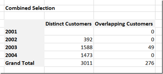
Notice that, thanks to the power of Power Pivot, customers are not double-counted in the new combined selection report on the right-hand side. For example, in 2003 841 customers bought one or more products selected in the slicer Product Selection A while in 2003 796 customers bought one or more products listed in the slicer Product Selection B. 841+796=1637, but in the combined selection report correctly states that only 1588 distinct customers bought products listed in either Selection A or Selection B. We can use these numbers to do one final, useful calculation: 1637-1588=49, so there were 49 customers who must have bought products in both Selection A and Selection B. The formula to do this is pretty straightforward and looks like this:

=IFERROR(($C19+$G19)-$J19, 0)

You can download the sample workbook for this post here.

Chris has been working with Microsoft BI tools since he started using beta 3 of OLAP Services back in the late 90s. Since then he has worked with Analysis Services in a number of roles (including three years spent with Microsoft Consulting Services) and he is now an independent consultant specialising in complex MDX, Analysis Services cube design and Analysis Services query performance problems. His company website can be found at http://www.crossjoin.co.uk and his blog can be found at http://cwebbbi.wordpress.com/ .