PowerPivot Top N Reports Using Excel Cube Formulas

Reposted from Chris Webb's blog with the author's permission.

Top N reports are an extremely common requirement: my customers are always trying to find their top 10 products or sales people or geographies by some measure or other. Luckily this type of report is fairly easy to build in PowerPivot if you’re using a PivotTable; in fact, Rob Collie wrote a good blog post on this subject only last week which is well worth a read. The problem with PivotTables is, however, that they are a pain to format and many people prefer to use Excel cube formulas for their dashboards – and unfortunately dynamic Top N reports are surprisingly difficult to implement with cube formulas. As the discussions here and here show, even when you’re using CubeSet and CubeRankedMember you need to know MDX pretty well and even then it’s a bit messy. Here, instead, is a pure DAX solution to the problem which, while not as simple as I’d like, involves no MDX, no clever use of Excel cube functions, and works when you select more than one item in a slicer.

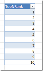
The first thing you need to do is to create a table with as many rows in as you need items in your Top N report. In my example I’m going to return the top 10 products in a model built from the Adventure Works database, so here’s my table (called TopNRank):

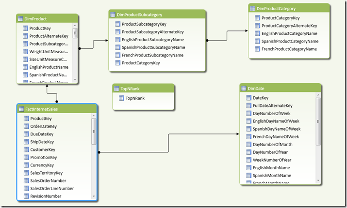
Here’s my model in Diagram View:

And here’s a screenshot of my main worksheet, for reference, with two Slicers on CalendarYear and EnglishProductCategoryName; a PivotTable with a Top 10 filter applied on EnglishProductName (to check the output and for debugging); and below it my Excel formulas, with the ten values from the TopNRank table on rows and two measures called [TopN Product Name] and [TopN Product Sales] on columns, showing the same top 10 values:

Step 1 is to create a measure called [Sales] that simply sums up the values in the [Sales Amount] column:

Sales:=SUM([SalesAmount])

You can then create a measure, called [Product Rank] here (and shown in the PivotTable above), that returns the rank of each product by [Sales] for the current year and category:

Product Rank:=
IF(
ISBLANK([Sales])
, BLANK()
, RANKX(ALL(DimProduct[EnglishProductName]), [Sales], [Sales], 0, Dense)
)

The basic idea for this approach is that with the Excel cube formulas, you’re going to use the values from the TopNRank table on rows and then use a measure to return the name of the top Nth Product for each row. This measure needs to return the name of the product that has the same rank value as whichever value from the TopNRank table is on rows. For example, in the screenshot above, in cell D21 there is a CubeMember function that returns the value 1 from TopNRank table; in cell D22 there is a CubeValue function that references the new measure, and this filters the list of all Products to return the name of the Product where [Product Rank] is 1, which is Road-150 Red, 48 (as you can see from the PivotTable).

There’s a problem with this approach, however, and that is that the RankX function always returns tied ranks when two products have the same value for [Sales]. So, in the PivotTable in the screenshot above, there are two products with the rank 2 because they have the same value for the [Sales] measure – and this causes big problems for the approach described in the previous paragraph. Despite what BOL says you can’t calculate a rank by more than one column, so the only way to get around this is to ensure that tied ranks can never occur, and the way I’ve done this is to rank by [Sales] and the name of the product by using the following measures:

Product Name:=
FIRSTNONBLANK(VALUES(DimProduct[EnglishProductName]), DimProduct[EnglishProductName])

Product Name Rank:=
IF(
ISBLANK([Sales])
, BLANK()
, RANKX(ALL(DimProduct[EnglishProductName]),[Product Name])
)

Combined Rank:=
[Product Rank] + (1/[Product Name Rank])

Untied Product Rank:=
RANKX(ALL(DimProduct[EnglishProductName]), [Combined Rank],,1)

With this done, at long last it’s possible to create the measure that returns the name of the Top Nth product as follows:

TopN Product Name:=
IF(
ISFILTERED(‘TopNRank’[TopNRank]) && ISBLANK([Sales])=FALSE()
, FIRSTNONBLANK(
FILTER(VALUES(DimProduct[EnglishProductName])
, [Untied Product Rank]=VALUES(‘TopNRank’[TopNRank]))
, DimProduct[EnglishProductName])
, BLANK()
)

And here’s the measure that returns the value of [Sales] for each product:

TopN Product Sales:=
IF(
ISFILTERED(‘TopNRank’[TopNRank]) && ISBLANK([Sales])=FALSE()
, CALCULATE(
SUM(FactInternetSales[SalesAmount])
, FILTER(
VALUES(DimProduct[EnglishProductName])
, DimProduct[EnglishProductName]=[TopN Product Name]))
, BLANK()
)

I’ve been told by the customer that implemented this approach that performance on larger models, while acceptable, is a bit slow and that it gets worse the more items you display in your top n list. This doesn’t surprise me and to be honest I’ll need to do some experiments to see if I can improve performance.

You can download my sample workbook (Excel 2010 64 bit, PowerPivot V2.0) from here.

Chris has been working with Microsoft BI tools since he started using beta 3 of OLAP Services back in the late 90s. Since then he has worked with Analysis Services in a number of roles (including three years spent with Microsoft Consulting Services) and he is now an independent consultant specialising in complex MDX, Analysis Services cube design and Analysis Services query performance problems. His company website can be found at http://www.crossjoin.co.uk and his blog can be found at http://cwebbbi.wordpress.com/ .