Row Selection Using Slicers in PowerPivot - Part 1
Reposted from Jason Thomas blog with the author's permission.
A couple of months back, I had written a post on ‘Measure selection using Slicers in PowerPivot’ and this turned out to be one of my most popular ones in the PowerPivot / DAX category. It was just a matter of time before someone asked how to do the same with rows or dimension attributes using slicers in PowerPivot. And the case supporting it is also becoming strong with more and more dashboards being built in Power View and Excel. Well, as usual, this functionality is not available out of the box but you could simulate it with a little change to your data model. Read on for the solution.
I will be first briefly explain the solution pattern and then apply it to a couple of scenarios.
Solution
1) A new table should be built and added to the existing data model. The new table should have at least 3 columns
- GroupName : the text displayed in the slicers (for e.g., Product, Customer, etc.)
- GroupValue : the actual values that should be displayed in the rows on selecting the slicer values (for e.g., if Product is selected in the slicer for GroupName, then GroupValues will be the Product values)
- Grain of the Tables : If all the GroupNames displayed in the slicer belong to the same dimension (for eg, Product, Category and SubCategory in the Product dimension), then only one column is required which would be the grain of the dimension (to be precise, the column of the table linked to the facts which is usually the grain of the dimension). If multiple dimensions are involved in the GroupNames (for eg, Product and Customer), then the number of columns increases based on the grain of the participating dimensions.For each GroupName, all valid combinations of GroupValue and Grain columns should be generated.
2) The grain columns should then be related to the dimensions.
3) Create new calculated measures for each of the required measure by passing the new table in the filter part of a calculate statement and then use them in the pivot tables or charts.
Scenario I - GroupNames in one dimension and 1-to-Many Relationship
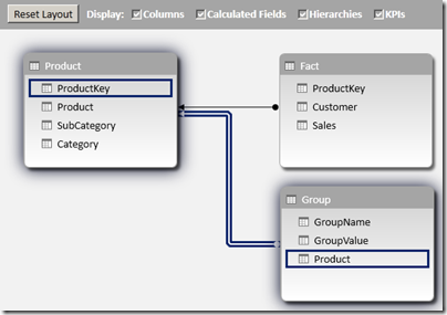
Our data model for this scenario will have a Product table and a Fact table which shows the sales by Product and Customer. The Product table has ProductKey, Product, SubCategory and Category columns. Our requirement is that we should be able to select Product, SubCategory or Category in the slicers and display the selected values on the row of the pivot table.
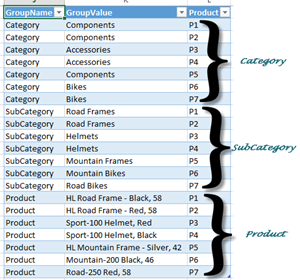
1) As per the solution steps, we will have to create a new table as shown below
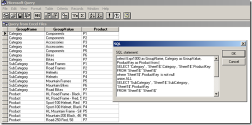
Since the slicers need to display the three levels, the GroupName values will be Category, SubCategory and Product. The granularity is at the Product level and hence that will be the third column. Note that for each value in GroupName, there should be a row mapping the GroupValue to the grain column (which is Product here). This sort of table is very easy to create if the source is a relational database. For this demo, I used linked tables and hence to automate the creation of this table, I had to use Microsoft Query as a datasource to pull data from the linked tables.
SELECT Expr1000 AS GroupName, Category AS GroupValue, ProductKey AS Product FROM (
SELECT 'Category' , 'Sheet1$'.Category , 'Sheet1$'.ProductKey
FROM 'Sheet1$' 'Sheet1$'
WHERE 'Sheet1$'.ProductKey IS NOT NULL
UNION ALL
SELECT 'SubCategory' , 'Sheet1$'.SubCategory , 'Sheet1$'.ProductKey
FROM 'Sheet1$' 'Sheet1$'
WHERE 'Sheet1$'.ProductKey IS NOT NULL
UNION ALL
SELECT 'Product' , 'Sheet1$'.Product , 'Sheet1$'.ProductKey
FROM 'Sheet1$' 'Sheet1$'
WHERE 'Sheet1$'.ProductKey IS NOT NULL
)
(Please note that I am not a MS query datasource expert and I had to workaround getting the column alias names by bringing the outermost select statement. This should have been a simple UNION ALL in SQL Server). If there is any data change in the linked tables, the Refresh button should be clicked twice in the Excel window (so that the Query can populate the changed data in the new table as well as refresh the PowerPivot model with the changed data).
2) Add this new table (Group) to the data model and then relate the Product column in this table to the ProductKey column in the Product table.
3) Hide the original measure Sales, and then create a new measure with the formula given below
NewSales:=CALCULATE(SUM(Fact[Sales]), 'Group')
4) Check out the results by creating a pivot table with GroupValue on the rows, NewSales on Values and GroupName in Slicers.
Download the Excel 2013 file with the solution from here.
Scenario II - GroupNames in one dimension and Many-to-Many Relationship
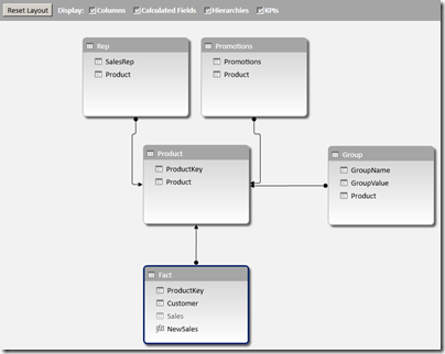
Our data model for this scenario will have a Product table, Fact table which shows the sales which shows the sales by Product and Customer, and two tables – Sales Rep and Promotions which will have a many to many relationship with Product.
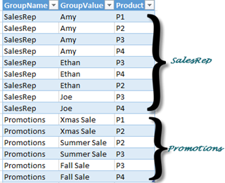
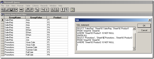
1) The Group table should have the below format
To create the Group table, we again use Microsoft Query as a datasource to pull data from the linked tables.
SELECT Expr1000 AS GroupName, SalesRep AS GroupValue, Product1 AS Product FROM (
SELECT 'SalesRep', `Sheet1$`.SalesRep, `Sheet1$`.Product1
FROM `Sheet1$` `Sheet1$`
WHERE `Sheet1$`.Product1 IS NOT NULL
UNION ALL
SELECT 'Promotions' , `Sheet1$`.Promotions , `Sheet1$`.Product2
FROM `Sheet1$` `Sheet1$`
WHERE `Sheet1$`.Product2 IS NOT NULL
)
2) Add this new table (Group) to the data model and then relate the Product column in this table to the ProductKey column in the Product table.
3) Hide the original measure Sales, and then create a new measure with the formula given below
NewSales:=CALCULATE(sum(Fact[Sales]), 'Group', 'Promotions', 'Rep')
4) Check out the results by creating a pivot table with GroupValue on the rows, NewSales on Values and GroupName in Slicers.
Download the Excel 2013 file with the solution from here.
I have got two more scenarios to show but guess that will have to wait till the second part of this series.
Note
There are some unique concepts here which might raise questions like
- why didn't I use DAX queries to seed my Group table? Well, I couldn't find a easy way to do union in DAX and that is the reason why I used MS query. It might not be the best way but it sure is an option.
- Is there any other way to avoid the double refresh of the file? I couldn't find any other option to do so (actually, you will need to do that even if you are using DAX queries to seed the Group table). That is, if you are avoiding VBA. Javier Guillen has promised to write a quick post on how to do it with a single refresh using VBA.
 | Jason has been working with Microsoft BI tools since he joined the IT industry in 2006. Since then he has worked across SSAS, SSRS and SSIS for a large number of clients like Unilever, Imperial Tobacco, IATA, Schneider Electric, etc. He is currently working at MindTree Ltd, Bangalore (www.mindtree.com) and his personal blog site can be found at http://www.sqljason.com His blogs can also be found at the popular technical site BeyondRelational.com at http://beyondrelational.com/blogs/jason |

