Optimising SSAS Many-To-Many Relationships By Adding Redundant Dimensions

Reposted from Chris Webb's blog with the author's permission.

The most elegant way of modelling your SSAS cube doesn't always give you the best query performance. Here's a trick I used recently to improve the performance of a many-to-many relationship going through a large fact dimension and large intermediate measure group.

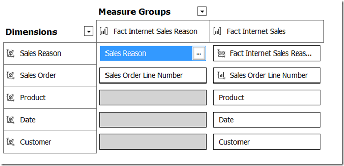
Consider the following cube, built from the Adventure Works DW database and showing a many-to-many relationship:

The Fact Internet Sales measure group contains sales data; the Product, Date and Customer dimensions are what you would expect; Sales Order is a fact dimension with one member for each sales transaction and therefore one member for each row in the fact table that Fact Internet Sales is built from. Each Sales Order can be associated with zero to many Sales Reasons, and the Sales Reason dimension has a many-to-many relationship with the Fact Internet Sales measure group through the Fact Internet Sales Reason measure group. Only the Sales Order dimension connects directly to both the Fact Internet Sales Reason and Fact Internet Sales measure groups.

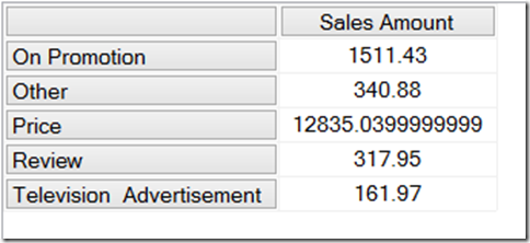
There's nothing obviously wrong with the way this is modelled - it works and returns the correct figures – and the following query shows how the presence of the many-to-many relationship means you can see the Sales Amount measure (from the Fact Internet Sales measure group) broken down by Sales Reason:

 
 select {[Measures].[Sales Amount]} on 0, non empty [Sales Reason].[Sales Reason].[Sales Reason].members on 1 from m2m1 where([Date].[Calendar Year].&[2003],  [Product].[Product Category].&[3], [Customer].[Country].&[United Kingdom]) 
 

However, to understand how we can improve the performance of a many-to-many relationship you have to understand how SSAS resolves the query internally. At a very basic level, in this query, SSAS starts with all of the Sales Reasons and then, for each one, finds the list of Sales Orders associated with it by querying the Fact Sales Reason measure group. Once it has the list of Sales Orders for each Sales Reason, it queries the Fact Internet Sales measure group (which is also filtered by the Year 2003, the Product Category Clothing and the Customer Country UK) and sums up the value of Sales Amount for those Sales Orders, getting a single value for each Sales Reason. A Profiler trace shows this very clearly:

The Resource Usage event gives the following statistics for this query:

READS, 7

READ_KB, 411

WRITES, 0

WRITE_KB, 0

CPU_TIME_MS, 15

ROWS_SCANNED, 87299

ROWS_RETURNED, 129466

Given that the Sales Order dimension is a large one (in this case around 60000 members - and large fact dimensions are quite common with many-to-many relationships) it's likely that one Sales Reason will be associated with thousands of Sales Orders, and therefore SSAS will have to do a lot of work to resolve the relationship.

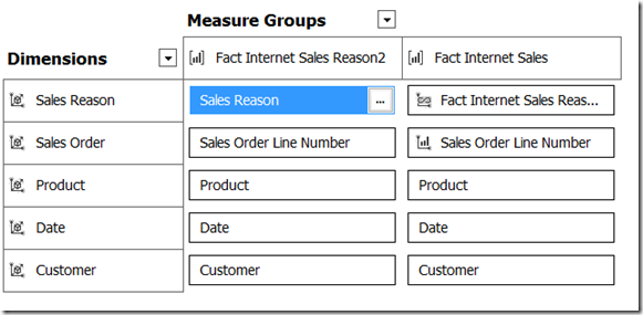
In this case, the optimisation comes with the realisation that in this case we can add the other dimensions present in the cube to the Fact Sales Reason measure group to try to reduce the number of Sales Orders that each Sales Reason is resolved to. Since Sales Order is a fact dimension, with one member for each sales transaction, then since each sales transaction also has a Date, a Product and a Customer associated with it we can add the keys for these dimensions to the fact table on which Fact Sales Reasons is built and join these dimensions to it directly:

This is not an assumption you can make for all many-to-many relationships, for sure, but it's certainly true for a significant proportion.

The Product, Date and Customer dimensions don't need to be present for the many-to-many relationship to work, but adding a Regular relationship between them and Fact Internet Sales Reason helps SSAS speed up the resolution of the many-to-many relationship when they are used in a query. This is because in the original design, in the test query the selection of a single member on Sales Reason becomes a selection on all of the Sales Orders that have ever been associated with that Sales Reason; with the new design, the selection of a single member on Sales Reason becomes a selection on a combination of Dates, Customers, Products and Sales Orders - and since the query itself is also applying a slice on Date, Customer and Product, this is a much smaller selection than before. For the query shown above, with the new design, the Resource Usage event now shows:

READS, 11

READ_KB, 394

WRITES, 0

WRITE_KB, 0

CPU_TIME_MS, 0

ROWS_SCANNED, 47872

ROWS_RETURNED, 1418

The much lower numbers for ROWS_SCANNED and ROWS_RETURNED shows that the Storage Engine is doing a lot less work. For the amount of data in Adventure Works the difference in query performance is negligible, but in the real world I've seen this optimisation make a massive difference to performance, resulting in queries running up to 15 times faster.

Don't forget that there are many other ways of optimising many-to-many relationships such as the those described in this white paper. Also, if you have a large fact dimension, if it does not need to be visible to the end user and is only needed to make the many-to-many relationship work, you can reduce the overhead of processing it by breaking it up into multiple smaller dimensions as described here.

Chris has been working with Microsoft BI tools since he started using beta 3 of OLAP Services back in the late 90s. Since then he has worked with Analysis Services in a number of roles (including three years spent with Microsoft Consulting Services) and he is now an independent consultant specialising in complex MDX, Analysis Services cube design and Analysis Services query performance problems. His company website can be found at http://www.crossjoin.co.uk and his blog can be found at http://cwebbbi.wordpress.com/ .