MDX Solve Order, SCOPE_ISOLATION and the Aggregate() function

Reposted from Chris Webb's blog with the author's permission.

Solve order in MDX is a mess. Back in the good old days of Analysis Services 2000 it was a difficult concept but at least comprehensible; unfortunately when Analysis Services 2005 was released a well-intentioned attempt at making it easier to work with in fact ended up making things much, much worse. In this post I'm going to summarise everything I know about solve order in MDX to try to make this complicated topic a little bit easier to understand.

If you're an experienced MDXer, at this point you'll probably lose interest because you think you know everything there is to know about solve order already. Up until two weeks ago that's what I though too, so even if you know everything I say in the first half of this post keep reading - there's some new stuff at the end I've only just found out about.

Let's start with a super-simple cube built from a single table, with two measures (Sales Amount and Cost Amount) and a Product dimension containing a single attribute hierarchy with two members (Apples and Oranges). Everything is built from the following table:

Solve Order and calculated members in the WITH clause

To understand what solve order is and how it can be manipulated, let's start off looking at an example that uses only calculated members in the WITH clause of a query. Consider the following:

WITH

MEMBER [Measures].[Cost %] AS

DIVIDE([Measures].[Cost Amount],[Measures].[Sales Amount]),

FORMAT_STRING='0.0%'

MEMBER [Product].[Product].[Total Fruit] AS

SUM({[Product].[Product].&[Apples],

[Product].[Product].&[Oranges]})

SELECT

{[Measures].[Sales Amount],

[Measures].[Cost Amount],

MEASURES.[Cost %]}

ON COLUMNS,

{[Product].[Product].&[Apples],

[Product].[Product].&[Oranges],

[Product].[Product].[Total Fruit]}

ON ROWS

FROM SALES

There are two calculated members here:

• Cost % divides Cost Amount by Sales Amount to find the percentage that costs make up of the sales amount
• Total Fruit sums up the values for Apples and Oranges

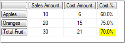
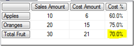
The output of the query is as follows:

Solve order controls the order that MDX calculations are evaluated when two or more of them overlap in the same cell. In this case Cost % and Total Fruit are both evaluated in the bottom right-hand cell; Total Fruit is calculated first, giving the values of 30 for Sales Amount and 21 for Cost Amount, and Cost % is calculated after that. The bottom right-hand cell is the only cell where these two calculations overlap and the only cell where solve order is relevant in this query.

In this case, 70% is the value you would expect to get. You, however, can control solve order for calculations in the WITH clause by setting the SOLVE_ORDER property for each calculated member, like so:

WITH

MEMBER [Measures].[Cost %] AS

DIVIDE([Measures].[Cost Amount],[Measures].[Sales Amount]),

FORMAT_STRING='0.0%',

SOLVE_ORDER=1

MEMBER [Product].[Product].[Total Fruit] AS

SUM({[Product].[Product].&[Apples],

[Product].[Product].&[Oranges]}),

SOLVE_ORDER=2

SELECT

{[Measures].[Sales Amount],

[Measures].[Cost Amount],

MEASURES.[Cost %]}

ON COLUMNS,

{[Product].[Product].&[Apples],

[Product].[Product].&[Oranges],

[Product].[Product].[Total Fruit]}

ON ROWS

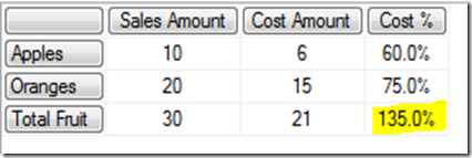
FROM SALES

Now the value in the bottom right-hand corner is 135% instead of 70%: Cost % is calculated first, then Total Fruit second so 60%+75%=135%. The SOLVE_ORDER property of a calculated member is an integer value, and the lower the SOLVE_ORDER value the earlier the calculation will be evaluated, so with Cost % having a solve order of 1 and Total Fruit having a solve order of 2, this forces Cost % to be calculated first now even though in this case it gives what is clearly an 'incorrect' result.

Solve Order and calculated members defined on the cube

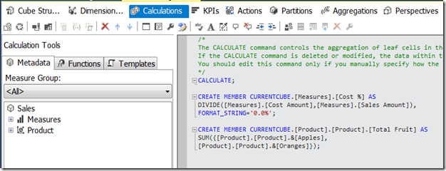
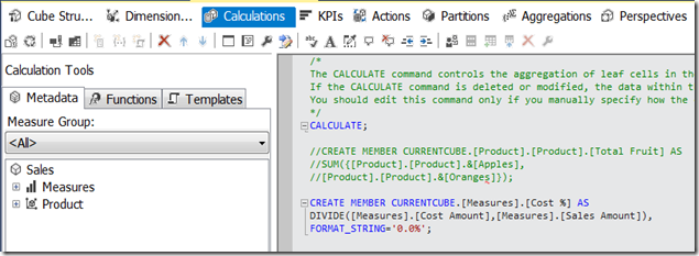
Things now get a bit more complicated. There's a different way of controlling solve order if your calculations are defined on the cube itself: in this case, solve order is determined by the order that the calculations appear on the Calculations tab. So if the calculations tab of the Cube Editor contains the calculations in this order:

CREATE MEMBER CURRENTCUBE.[Measures].[Cost %] AS

DIVIDE([Measures].[Cost Amount],[Measures].[Sales Amount]),

FORMAT_STRING='0.0%';

CREATE MEMBER CURRENTCUBE.[Product].[Product].[Total Fruit] AS

SUM({[Product].[Product].&[Apples],

[Product].[Product].&[Oranges]});

.and you run the following query:

SELECT

{[Measures].[Sales Amount],

[Measures].[Cost Amount],

MEASURES.[Cost %]}

ON COLUMNS,

{[Product].[Product].&[Apples],

[Product].[Product].&[Oranges],

[Product].[Product].[Total Fruit]}

ON ROWS

FROM SALES

You get the incorrect result again:

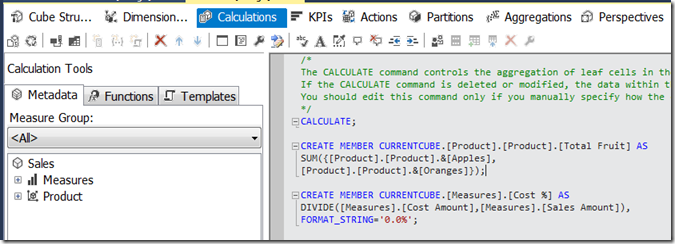
.but if you change the order of the calculations so that Total Fruit comes first:.and rerun the same query, you get the correct results:

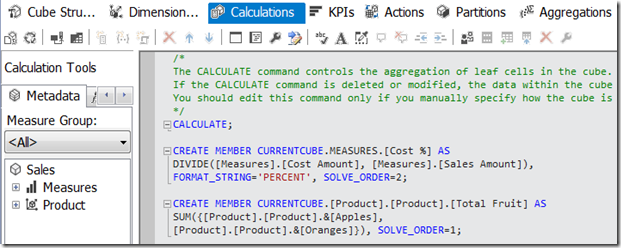
The SOLVE_ORDER property can also be used with calculations defined on the cube to override the effect of the order of calculations. So defining the following calculations on the cube:

CREATE MEMBER CURRENTCUBE.MEASURES.[Cost %] AS

DIVIDE([Measures].[Cost Amount], [Measures].[Sales Amount]),

FORMAT_STRING='PERCENT', SOLVE_ORDER=2;

CREATE MEMBER CURRENTCUBE.[Product].[Product].[Total Fruit] AS

SUM({[Product].[Product].&[Apples],

[Product].[Product].&[Oranges]}), SOLVE_ORDER=1;

.means that, even though Total Fruit comes after Cost % on the Calculations tab, because it has a lower solve order set using the SOLVE_ORDER property it is evaluated before Cost % and the query still returns the correct value:

Solve order and calculations defined in the WITH clause and on the cube

What happens if some calculations are defined on the cube, and some are defined in the WITH clause of a query? By default, calculations defined on the cube always have a lower solve order than calculations defined in the WITH clause of a query; the SOLVE_ORDER property has no effect here. So if Total Fruit is defined in the WITH clause and Cost % on the cube, you get the incorrect result:

WITH

MEMBER [Product].[Product].[Total Fruit] AS

SUM({[Product].[Product].&[Apples],

[Product].[Product].&[Oranges]})

SELECT

{[Measures].[Sales Amount],

[Measures].[Cost Amount],

MEASURES.[Cost %]}

ON COLUMNS,

{[Product].[Product].&[Apples],

[Product].[Product].&[Oranges],

[Product].[Product].[Total Fruit]}

ON ROWS

FROM SALES

Of course, if Total Fruit is defined on the cube and Cost % is defined in the WITH clause you will get the correct answer. However, usually measures like Cost % are defined on the cube and it's calculations like Total Fruit, which define custom groupings, that are defined on an ad hoc basis in the WITH clause. This is a problem.

The SCOPE_ISOLATION property

This default behaviour of calculations defined on the cube always having a lower solve order than calculations in the WITH clause can be overridden using the SCOPE_ISOLATION property. Setting SCOPE_ISOLATION=CUBE for a calculated member defined in the WITH clause will give that calculated member a lower solve order than any calculations defined on the cube. So, with Cost % still defined on the cube the following query now gives the correct results:

WITH

MEMBER [Product].[Product].[Total Fruit] AS

SUM({[Product].[Product].&[Apples],

[Product].[Product].&[Oranges]}),

SCOPE_ISOLATION=CUBE

SELECT

{[Measures].[Sales Amount],

[Measures].[Cost Amount],

MEASURES.[Cost %]}

ON COLUMNS,

{[Product].[Product].&[Apples],

[Product].[Product].&[Oranges],

[Product].[Product].[Total Fruit]}

ON ROWS

FROM SALES

The Aggregate() function

Using the MDX Aggregate() function (and in fact also the VisualTotals() function - but you probably won't ever want to use it) inside a calculation has a similar effect to the SCOPE_ISOLATION property in that it forces a calculation to be evaluated at a lower solve order than anything else. Therefore, in the previous example, instead of using the SCOPE_ISOLATION property you can change the calculation to use the Aggregate() function instead of Sum() and get the correct results:

WITH

MEMBER [Product].[Product].[Total Fruit] AS

AGGREGATE({[Product].[Product].&[Apples],

[Product].[Product].&[Oranges]})

SELECT

{[Measures].[Sales Amount],

[Measures].[Cost Amount],

MEASURES.[Cost %]}

ON COLUMNS,

{[Product].[Product].&[Apples],

[Product].[Product].&[Oranges],

[Product].[Product].[Total Fruit]}

ON ROWS

FROM SALES

The general rule is, therefore, whenever you are creating custom-grouping type calculated members like Total Fruit in the WITH clause of a query, to use the Aggregate() function rather than Sum(). The fact that Aggregate() takes into account the AggregateFunction property of each measure on the cube (so that distinct count, min and max measures are dealt with correctly) is another good reason to use it.

Using the Aggregate() function in calculations defined on the cube has the same effect. Even when the Total Fruit calculated member is defined after Cost % on the Calculations tab, as here:

.so long as Total Fruit uses the Aggregate() function, running the test query gives the correct result:

SELECT

{[Measures].[Sales Amount],

[Measures].[Cost Amount],

MEASURES.[Cost %]}

ON COLUMNS,

{[Product].[Product].&[Apples],

[Product].[Product].&[Oranges],

[Product].[Product].[Total Fruit]}

ON ROWS

FROM SALES

There are some very interesting details about the way Aggregate() changes solve order though.

First of all, using the Aggregate() function in a calculated member doesn't change the solve order of the whole calculation, just the part of the calculation that uses the Aggregate() function. With the following calculations defined on the cube:

CREATE MEMBER CURRENTCUBE.[Measures].[Cost %] AS

DIVIDE([Measures].[Cost Amount],[Measures].[Sales Amount]),

FORMAT_STRING='0.0%';

CREATE MEMBER CURRENTCUBE.[Product].[Product].[One Aggregate] AS

AGGREGATE({[Product].[Product].&[Apples],

[Product].[Product].&[Oranges]});

CREATE MEMBER CURRENTCUBE.[Product].[Product].[One Sum] AS

SUM({[Product].[Product].&[Apples],

[Product].[Product].&[Oranges]});

CREATE MEMBER CURRENTCUBE.[Product].[Product].[Two Aggregates] AS

AGGREGATE({[Product].[Product].&[Apples],

[Product].[Product].&[Oranges]})

+

AGGREGATE({[Product].[Product].&[Apples],

[Product].[Product].&[Oranges]});

CREATE MEMBER CURRENTCUBE.[Product].[Product].[Two Sums] AS

SUM({[Product].[Product].&[Apples],

[Product].[Product].&[Oranges]})

+

SUM({[Product].[Product].&[Apples],

[Product].[Product].&[Oranges]});

CREATE MEMBER CURRENTCUBE.[Product].[Product].[One Aggregate One Sum] AS

AGGREGATE({[Product].[Product].&[Apples],

[Product].[Product].&[Oranges]})

+

SUM({[Product].[Product].&[Apples],

[Product].[Product].&[Oranges]});

.running the following query:

SELECT

{[Measures].[Sales Amount],

[Measures].[Cost Amount],

MEASURES.[Cost %]}

ON COLUMNS,

{[Product].[Product].&[Apples],

[Product].[Product].&[Oranges],

[Product].[Product].[One Aggregate],

[Product].[Product].[One Sum],

[Product].[Product].[Two Aggregates],

[Product].[Product].[Two Sums],

[Product].[Product].[One Aggregate One Sum]}

ON ROWS

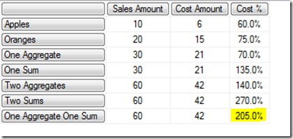
FROM SALES

.gives these results:

The value returned for the calculation [One Aggregate One Sum], which contains an Aggregate() and a Sum(), shows that the value returned by the Aggregate() is evaluated at a different solve order than the value returned by Sum(), even if they are inside the same calculated member.

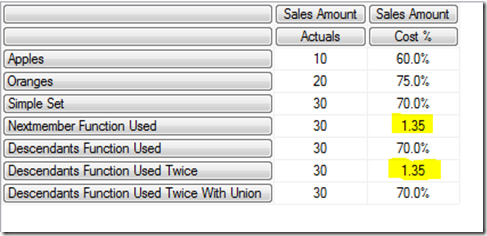
Furthermore, in some very obscure cases the contents of the set passed to the Aggregate() function determine whether its special solve order behaviour happens or not. I don't know for sure what all those cases are but I have seen this happen with time utility (aka date tool aka shell) dimensions. Here's an example.

The demo cube I've been using in this post has been changed to add a new dimension, called Data Type, which has just one hierarchy with one member on it called Actuals; Data Type is a fairly standard time utility dimension. The Cost % calculation has also been changed so that it's now a calculated member on the Data Type dimension, although it is still defined on the cube. Here's its new definition:

CREATE MEMBER CURRENTCUBE.[Data Type].[Data Type].[Cost %] AS

DIVIDE(

([Measures].[Cost Amount],[Data Type].[Data Type].&[Actuals]),

([Measures].[Sales Amount],[Data Type].[Data Type].&[Actuals])),

FORMAT_STRING='0.0%';

Now if I run the following query:

WITH

MEMBER [Product].[Product].[Simple Set] AS

AGGREGATE({[Product].[Product].&[Apples],

[Product].[Product].&[Oranges]})

MEMBER [Product].[Product].[Nextmember Function Used] AS

AGGREGATE({[Product].[Product].&[Apples],

[Product].[Product].&[Apples].NEXTMEMBER})

MEMBER [Product].[Product].[Descendants Function Used] AS

AGGREGATE(DESCENDANTS({[Product].[Product].&[Apples],

[Product].[Product].&[Oranges]}))

MEMBER [Product].[Product].[Descendants Function Used Twice] AS

AGGREGATE({

DESCENDANTS([Product].[Product].&[Apples]),

DESCENDANTS([Product].[Product].&[Oranges])

})

MEMBER [Product].[Product].[Descendants Function Used Twice With Union] AS

AGGREGATE(

UNION(

DESCENDANTS([Product].[Product].&[Apples]),

DESCENDANTS([Product].[Product].&[Oranges])

))

SELECT

{[Measures].[Sales Amount]}

*

[Data Type].[Data Type].ALLMEMBERS

ON COLUMNS,

{[Product].[Product].&[Apples],

[Product].[Product].&[Oranges],

[Product].[Product].[Simple Set],

[Product].[Product].[Nextmember Function Used],

[Product].[Product].[Descendants Function Used],

[Product].[Product].[Descendants Function Used Twice],

[Product].[Product].[Descendants Function Used Twice With Union]}

ON ROWS

FROM [Sales With Data Type]

I get these results:

Note that for some of the calculations, the Aggregate() function results in a lower solve order in the way we've already seen, but not for all of them. Using the NextMember() function, or having two Descendants() functions without wrapping them in a Union() function, seems to stop SSAS assigning the calculation a lower solve order. Ugh. Luckily, though, I have only been able to replicate this with calculated members from two non-measures dimensions; if Cost % is a calculated measure Aggregate() always gives the lower solve order. Apparently this is something that SSAS does on purpose to try to recognise 'visual total'-like calculated members and make them work the way you want automatically. This is definitely something to beware of if you are using time utility dimensions and calculations on other dimensions though, as it may result in incorrect values being displayed or performance problems if you're not careful.

[Thanks to Gabi Münster for showing me how Aggregate() works with different sets and Marius Dumitru for confirming that this is intended behaviour]

Chris has been working with Microsoft BI tools since he started using beta 3 of OLAP Services back in the late 90s. Since then he has worked with Analysis Services in a number of roles (including three years spent with Microsoft Consulting Services) and he is now an independent consultant specialising in complex MDX, Analysis Services cube design and Analysis Services query performance problems. His company website can be found at http://www.crossjoin.co.uk and his blog can be found at http://cwebbbi.wordpress.com/ .