Changing Granularity of Leaf Level Calculations in SSAS Tabular

Reposted from Jason Thomas blog with the author's permission.

My company is awesome!!! Everyday that I go to work, I discover something new and exciting from the people around me and come back home thinking – wow, today was just legendary! The best part of the day is when I get to discuss ideas with my colleagues, it is so fulfilling intellectually. So last month, I was having one of those discussions with PowerPivot/Tabular expert and my colleague, Javier Guillen (blog | twitter) on Last Non Empty functionality in multi-dimensional and one thing led to the other. Before we knew, we had discussed a lot of interesting things in both multi-dimensional and tabular about the Last Non Empty functionality and I am pretty sure that you will hear a lot on that field from us soon. Meanwhile, I decided to blog a quick post on one of the basic principles that we will be using for that.

Leaf level calculations in multi-dimensional usually impact the performance and hence, are advised to be done in the ETL part. You might be lucky to get away with such sort of calculations in your DSV also as named calculations. But changing the granularity of such calculations from leaf level to an intermediate level usually requires it to be done in the ETL if we are using the multi-dimensional mode (unless you want to impact the performance by a Scope statement or god forbid, a cross join in the calculation script). In scenarios like prototyping where we are still discovering about the data, changing the granularity of the calculations can be expected and it implies a lot of time lost in re-working the ETL. That is where the Tabular mode is such a big boon and I will be illustrating that fact in the following example.

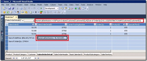
Consider the AdventureWorks database where there is Order Quantity for the Products and Customers, and the client would like to see the distribution of products across the customers. Now you can make a simple numerical distribution measure which is the number of customers that have data for that product by the total number of customer.

The DAX formula is given below

NumericalDistribution:=100 * SumX (
Values ( Customer[CustomerID] ),
If ( [Sum of OrderQty] > 0, 1, 0 )
) / DistinctCount (
Customer[CustomerID]
)

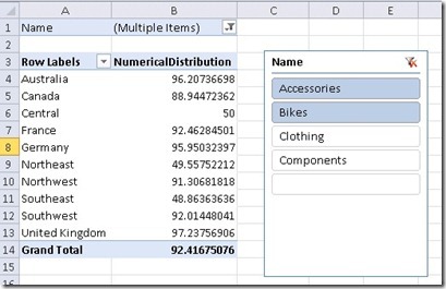
Let us look at the results when I analyze the same measure for all the Territories filtered by the Category – Accessories and Bikes

Now, let us assume a hypothetical situation where the goal of this year for the Country Sales Managers is to make their customers buy different products and the client wants to analyze the performance of the Sales Managers based on a new Distribution KPI. The numerical distribution measure is not a good indicator for this as it just checks whether the customer has order quantity or not for either Accessories or Bikes. A better indicator might be to assign a weight to each customer based on the different number of products that has order quantity by the total number of products. The formula for the new distribution is given below

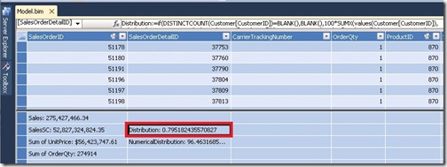
The new distribution takes the sum of weights for each customer and divides it by the total number of customer. The DAX formula for the same is given below

Distribution:=If (
DistinctCount ( Customer[CustomerID] ) = Blank ( ),
Blank ( ),
100 * SumX (
Values ( Customer[CustomerID] ),
Calculate (
DistinctCount ( SalesOrderDetail[ProductID] )
) / DistinctCount ( Product[ProductID] )
) / DistinctCount ( Customer[CustomerID] )
)

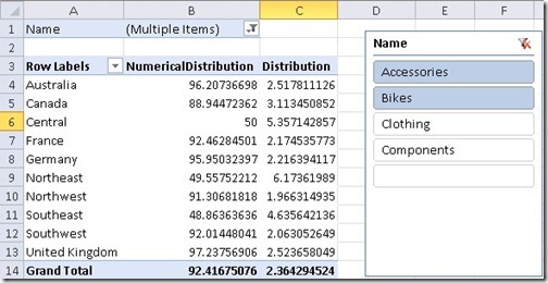
The results for the above formula is given below

We can see that the distribution values have become very low because of the low weight, as it is almost impossible to expect a customer to buy every product. So the client can come back and ask to calculate the distribution at the level of the Country instead of Customer. This will ensure that the distribution is more appropriately calculated. The new formula for the distribution will become

The DAX formula is given below

Distribution:=If (
DistinctCount ( SalesTerritory[CountryRegionCode] ) = Blank ( ),
Blank ( ),
100 * SumX (
Values ( SalesTerritory[CountryRegionCode]),
Calculate (
DistinctCount ( SalesOrderDetail[ProductID] )
) / DistinctCount ( Product[ProductID] )
) / DistinctCount ( SalesTerritory[CountryRegionCode] )
)

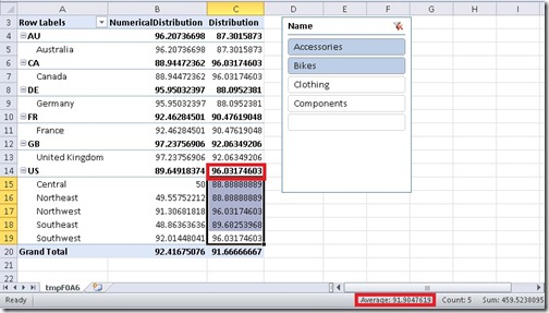
The results for the Distribution formula with the changed granularity analyzed by Country Code and Territory Name is given below

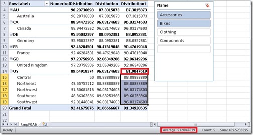
Now, the client may again come back and ask for the formula to be re-calculated on a territory level, as that looks more appropriate for them after seeing the data. Take the case of US for example. The distribution value for US is 96.03 but the average distribution based on the territories is 91.90. So the changed formula is shown below

The DAX formula is given below

Distribution1:=If (
DistinctCount ( SalesTerritory[Name] ) = Blank ( ),
Blank ( ),
100 * SumX (
Values ( SalesTerritory[Name]),
Calculate (
DistinctCount ( SalesOrderDetail[ProductID] )
) / DistinctCount ( Product[ProductID] )
) / DistinctCount ( SalesTerritory[Name] )
)

The result of the formula is given below and we can see that the new values takes the average from the territories at the country level.

Now after making all these changes, the client is happy with the end results. The important thing to note here is that we had this whole hypothetical process completed within half an hour and not days. Consider how much time we would have required to accomplish this in the multi-dimensional mode! Now if you are still in the mood for more DAX after this, make sure that you run by Javier’s latest blog where he uses a similar technique to mimic the MDX Scope behavior in DAX.